Step response of a first order system with derivative input contribution Matlab

The response of a system to a sudden excitation is often modeled as a step response. The following is an example of how to obtain the step response of a simple system. It illustrated the difference between a system with and without so-called numerator dynamics. Such dynamics represent an interaction due to velocity induced forces, such as those in viscous fluid dynamics or caused by a dashpot (also fluid-driven).

Consider the transfer function of a system given by

\begin{equation*} 4\dot{x}+x=g(t)+\dot{g}(t) \end{equation*}

\begin{equation*} T(s)=\frac{s+1}{4s+1} \end{equation*}

while for a second system given by

\begin{equation*} 4\dot{x}+x=g(t) \end{equation*}

\begin{equation*} T(s)=\frac{1}{4s+1} \end{equation*}

Find the response to an input of \(5u(t)\).

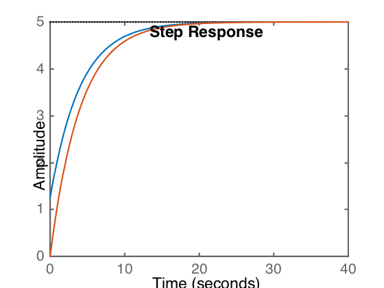
Given that the amplitude of the step input is 5, it's easiest to simply multiply the transfer function by five and use a unit step function, allowing us to use the Matlab step function.

sys1=tf([1 1]*5,[4 1])
sys2 = tf([1]*5,[4 1])
step(sys1);
hold on;
step(sys2)

sys1 =

  5 s + 5
  -------
  4 s + 1

Continuous-time transfer function.


sys2 =

     5
  -------
  4 s + 1

Continuous-time transfer function.

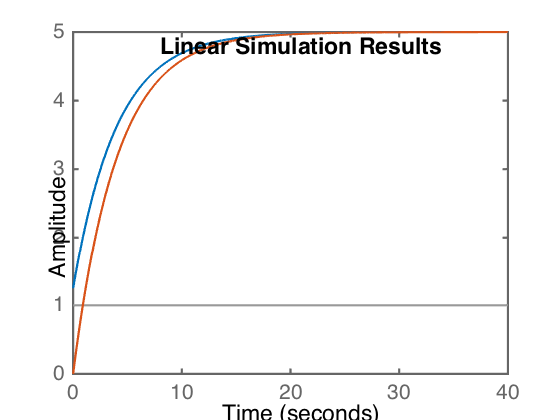
Alternatively, using lsim.

sys1=tf([1 1]*5,[4 1])
sys2 = tf([1]*5,[4 1])
t=0:.01:40;
u=t*0+1;
lsim(sys1,u, t);
hold on;
lsim(sys2,u,t)

My hand drawn free body diagrams and equations.

sys1 =

  5 s + 5
  -------
  4 s + 1

Continuous-time transfer function.


sys2 =

     5
  -------
  4 s + 1

Continuous-time transfer function.

In both cases, the blue line represents the sys1 response, and the orange line the sys2 response. This can be demonstrated by plotting them individually.

The effect of the \(\dot{g}(t)\) term is to effectively jump start the response at a higher level, equivalent to 5/4, which are two numbers you should see in the sys1 transfer function.

Comments