Mousai: An Open-Source General Purpose Harmonic Balance Solver

ASME Dayton Engineering Sciences Symposium 2017

Joseph C. Slater, October 23, 2017

%matplotlib inline
%load_ext autoreload
%autoreload 2
import scipy as sp
import numpy as np
import matplotlib.pyplot as plt
import matplotlib
import mousai as ms
from scipy import pi, sin
matplotlib.rcParams['figure.figsize'] = (11, 5)
from traitlets.config.manager import BaseJSONConfigManager
path = "/Users/jslater/anaconda3/etc/jupyter/nbconfig"
cm = BaseJSONConfigManager(config_dir=path)
cm.update("livereveal", {
              "theme": "sky",
              "transition": "zoom",
})

The autoreload extension is already loaded. To reload it, use:
  %reload_ext autoreload

{'theme': 'sky', 'transition': 'zoom'}

Overview

A wide array of contemporary problems can be represented by nonlinear ordinary differential equations with solutions that can be represented by Fourier Series:

• Limit cycle oscillation of wings/blades

• Flapping motion of birds/insects/ornithopters

• Flagellum (threadlike cellular structures that enable bacteria etc. to swim)

• Shaft rotation, especially including rubbing or nonlinear bearing contacts

• Engines

• Radio/sonar/radar electronics

• Wireless power transmission

• Power converters

• Boat/ship motions and interactions

• Cardio systems (heart/arteries/veins)

• Ultrasonic systems transversing nonlinear media

• Responses of composite materials or materials with cracks

• Near buckling behavior of vibrating columns

• Nonlinearities in power systems

• Energy harvesting systems

• Wind turbines

• Radio Frequency Integrated Circuits

• Any system with nonlinear coatings/friction damping, air damping, etc.

These can all be observed in a quick literature search on ‘Harmonic Balance’.

Why (did I) write Mousai?

• The ability to code harmonic balance seems to be publishable by itself

  • It’s not research- it’s just application of a known family of technique

• A limited number of people have this knowledge and skill

  • Most cannot access this technique

  • “Research effort” is spent coding the technique, not doing research

Why write Mousai? (continued)

• Matlab command eig unleashed power to the masses

  • Very few papers are published on eigensolutions- they have to be better than eig

  • eig only provides simple access to high-end eigensolvers written in C and Fortran

  • Undergraduates with no practical understanding of the algorithms easily solve problems that were intractable a few decades ago.

  • Access and ease of use of such techniques enable greater science and greater research.

  • The real world is nonlinear, but linear analysis dominates because the tools are easier to use.

  • With Mousai, an undergraduate can solve a nonlinear harmonic response problem easier then a PhD can today.

Theory:

Linear Solution

• Most dynamics systems can be modeled as a first order differential equation

\begin{equation}\ddot{\mathbf{z}}(t)=\mathbf{f}(\mathbf{z}(t),\mathbf{u}(t))\end{equation}

- Use finite differences
- Use Galerkin methods (Finite Elements)
- Of course- discrete objects

• This is the common State-Space form: -solutions exceedingly well known if it is linear

• Finding the oscillatory response, after dissipation of the transient response, requires long time marching.

  • Without damping, this may not even been feasible.

  • With damping, tens, hundreds, or thousands of cycles, therefore thousands of times steps at minimum.

For a linear system in the frequency domain this is

\begin{equation}j\omega\mathbf{Z}(\omega)=\mathbf{f}(\mathbf{Z}(\omega),\mathbf{U}(\omega))\end{equation}

\begin{equation}j\omega\mathbf{Z}(\omega)=A\mathbf{Z}(\omega)+B\mathbf{U}(\omega)\end{equation}

where

\begin{equation}A = \frac{\partial \mathbf{f}(\mathbf{Z}(\omega),\mathbf{U}(\omega))}{\partial\mathbf{Z}(\omega)},\qquad B = \frac{\partial \mathbf{f}(\mathbf{Z}(\omega),\mathbf{U}(\omega))}{\partial\mathbf{U}(\omega)}\end{equation}

are constant matrices.

The solution is:

\begin{equation}\mathbf{Z}(\omega) = \left(Ij\omega-A\right)^{-1}B\mathbf{U}(\omega)\end{equation}

where the magnitudes and phases of the elements of \(\mathbf{Z}\) provide the amplitudes and phases of the harmonic response of each state at the frequency \(\omega\).

Nonlinear solution

• For a nonlinear system in the frequency domain we assume a Fourier series solution

\begin{equation}\mathbf{z}(t)=\lim_{N\to\infty}\sum_{n=-N}^{N}\mathbf{Z}_n e^{j n \omega t}\end{equation}

• \(N=1\) for a single harmonic. \(n=0\) is the constant term.

• This can be substituted into the governing equation to find \(\dot{\mathbf{z}}(t)\):

\begin{equation}\dot{\mathbf{z}}(t)=\mathbf{f}(\mathbf{z}(t),\mathbf{u}(t))\end{equation}

• This is actually a function call to a Finite Element Package, CFD, Matlab function, - whatever your solver uses to get derivatives

• We can also find \(\dot{\mathbf{z}}(t)\) from the derivative of the Fourier Series:

\begin{equation}\dot{\mathbf{z}}(t)=\lim_{N\to\infty}\sum_{n=-N}^{N}j n \omega\mathbf{Z}_n e^{j n \omega t}\end{equation}

• The difference between these methods is zero when \(\mathbf{Z}_n\) are correct.

\begin{equation}\mathbf{0} \approx\sum_{n=-N}^{N}j n\omega \mathbf{Z}_n e^{j n \omega t}-\mathbf{f}\left(\sum_{n=-N}^{N}\mathbf{Z}_n e^{j n \omega t},\mathbf{u}(t)\right)\end{equation}

• These operations are wrapped inside a function that returns this error

• This function is used by a Newton-Krylov nonlinear algebraic solver.

• Calls any solver in the SciPy family of solvers with the ability to easily pass through parameters to the solver and to the external derivative evaluator.

Examples:

Duffing Oscillator

\begin{equation}\ddot{x}+0.1\dot{x}+x+0.1 x^3=\sin(\omega t)\end{equation}

# Define our function (Python)
def duff_osc_ss(x, params):
    omega = params['omega']
    t = params['cur_time']
    xd = np.array([[x[1]],
                   [-x[0] - 0.1 * x[0]**3 - 0.1 * x[1] + 1 * sin(omega * t)]])
    return xd

# Arguments are name of derivative function, number of states, driving frequency,
# form of the equation, and number of harmonics

t, x, e, amps, phases = ms.hb_time(duff_osc_ss, num_variables=2, omega=.1,
                                 eqform='first_order', num_harmonics=5)
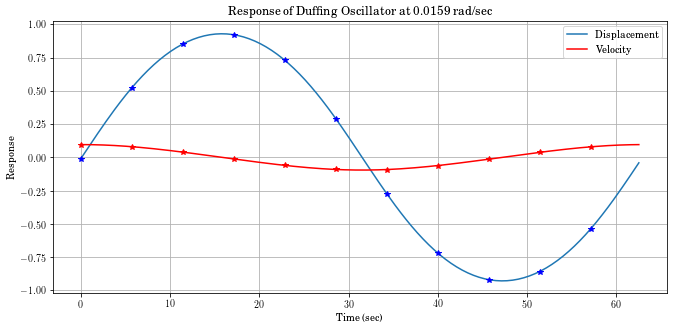
print('Displacement amplitude is ', amps[0])
print('Velocity amplitude is ', amps[1])

Displacement amplitude is  0.9469563546008394
Velocity amplitude is  0.09469563544416415

Mousai can easily recreate the near-continuous response

time, xc = ms.time_history(t, x)

def pltcont():
    time, xc = ms.time_history(t, x)
    disp_plot, _ = plt.plot(time, xc.T[:, 0], t,
                            x.T[:, 0], '*b', label='Displacement')
    vel_plot, _ = plt.plot(time, xc.T[:, 1], 'r',
                           t, x.T[:, 1], '*r', label='Velocity')
    plt.legend(handles=[disp_plot, vel_plot])
    plt.xlabel('Time (sec)')
    plt.title('Response of Duffing Oscillator at 0.0159 rad/sec')
    plt.ylabel('Response')
    plt.legend
    plt.grid(True)

fig=plt.figure()
ax=fig.add_subplot(111)
time, xc = ms.time_history(t, x)
disp_plot, _ = ax.plot(time, xc.T[:, 0], t,
                            x.T[:, 0], '*b', label='Displacement')
vel_plot, _ = ax.plot(time, xc.T[:, 1], 'r',
                           t, x.T[:, 1], '*r', label='Velocity')
ax.legend(handles=[disp_plot, vel_plot])
ax.set_xlabel('Time (sec)')
ax.set_title('Response of Duffing Oscillator at 0.0159 rad/sec')
ax.set_ylabel('Response')
ax.legend
ax.grid(True)

pltcont()# abbreviated plotting function

time, xc = ms.time_history(t, x)
disp_plot, _ = plt.plot(time, xc.T[:, 0], t,
                        x.T[:, 0], '*b', label='Displacement')
vel_plot, _ = plt.plot(time, xc.T[:, 1], 'r',
                       t, x.T[:, 1], '*r', label='Velocity')
plt.legend(handles=[disp_plot, vel_plot])
plt.xlabel('Time (sec)')
plt.title('Response of Duffing Oscillator at 0.0159 rad/sec')
plt.ylabel('Response')
plt.legend
plt.grid(True)

omega = np.arange(0, 3, 1 / 200) + 1 / 200
amp = sp.zeros_like(omega)
amp[:] = np.nan
t, x, e, amps, phases = ms.hb_time(duff_osc_ss, num_variables=2,
                                 omega=1 / 200, eqform='first_order', num_harmonics=1)
for i, freq in enumerate(omega):
    # Here we try to obtain solutions, but if they don't work,
    # we ignore them by inserting `np.nan` values.
    x = x - sp.average(x)
    try:
        t, x, e, amps, phases =
        ms.hb_time(duff_osc_ss, x0=x,
                 omega=freq, eqform='first_order', num_harmonics=1)
        amp[i] = amps[0]
    except:
        amp[i] = np.nan
    if np.isnan(amp[i]):
        break
plt.plot(omega, amp)

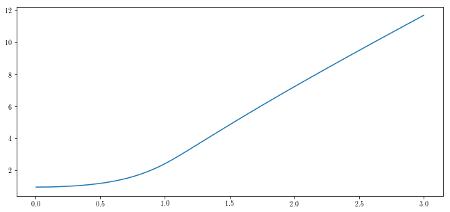
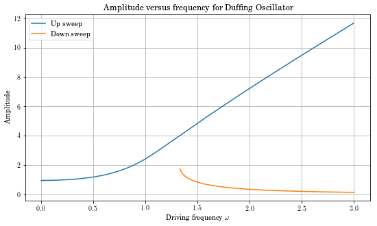
Let’s sweep through driving frequencies to find a frequency response function

omegal = np.arange(3, .03, -1 / 200) + 1 / 200
ampl = sp.zeros_like(omegal)
ampl[:] = np.nan
t, x, e, amps, phases = ms.hb_time(duff_osc_ss, num_variables=2,
                                 omega=3, eqform='first_order', num_harmonics=1)
for i, freq in enumerate(omegal):
    # Here we try to obtain solutions, but if they don't work,
    # we ignore them by inserting `np.nan` values.
    x = x - np.average(x)
    try:
        t, x, e, amps, phases = ms.hb_time(duff_osc_ss, x0=x,
                 omega=freq, eqform='first_order', num_harmonics=1)
        ampl[i] = amps[0]
    except:
        ampl[i] = np.nan
    if np.isnan(ampl[i]):
        break

plt.plot(omega,amp, label='Up sweep')
plt.plot(omegal,ampl, label='Down sweep')
plt.legend()
plt.title('Amplitude versus frequency for Duffing Oscillator')
plt.xlabel('Driving frequency $\\omega$')
plt.ylabel('Amplitude')
plt.grid()

Two degree of freedom system

\[\begin{split}\begin{bmatrix}1&0\\0&1\end{bmatrix}\begin{bmatrix}\ddot{x}_1\\ \ddot{x}_2\end{bmatrix}+\begin{bmatrix}2&-1 \\-1&2\end{bmatrix}\begin{bmatrix}{x}_1\\{x}_2\end{bmatrix}+\begin{bmatrix}\alpha x_{1}^{3}\\0\end{bmatrix}=\begin{bmatrix}0 \\A \sin(\omega t)\end{bmatrix}\end{split}\]

def two_dof_demo(x, params):
    omega = params['omega']
    t = params['cur_time']
    force_amplitude = params['force_amplitude']
    alpha = params['alpha']
    # The following could call an external code to obtain the state derivatives
    xd = np.array([[x[1]],
                   [-2 * x[0] - alpha * x[0]**3 + x[2]],
                   [x[3]],
                   [-2 * x[2] + x[0]]] + force_amplitude * np.sin(omega * t))
    return xd

Let’s find a response.

parameters = {'force_amplitude': 0.2}
parameters['alpha'] = 0.4
t, x, e, amps, phases = ms.hb_time(two_dof_demo, num_variables=4,
                                 omega=1.2, eqform='first_order', params=parameters)
amps

array([0.86696762, 0.89484597, 0.99030411, 1.04097851])

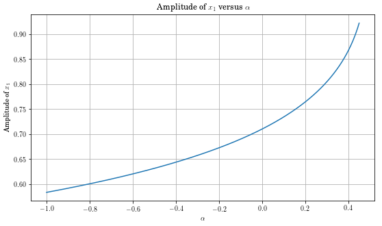
Or a parametric study of response amplitude versus nonlinearity.

alpha = np.linspace(-1, .45, 2000)
amp = np.zeros_like(alpha)
for i, alphai in enumerate(alpha):
    parameters['alpha'] = alphai
    t, x, e, amps, phases = ms.hb_time(two_dof_demo, num_variables=4, omega=1.2,
                                     eqform='first_order', params=parameters)
    amp[i] = amps[0]

plt.plot(alpha,amp)
plt.title('Amplitude of $x_1$ versus $\\alpha$')
plt.ylabel('Amplitude of $x_1$')
plt.xlabel('$\\alpha$')
plt.grid()

Two degree of freedom system with Coulomb Damping

\[\begin{split}\begin{bmatrix}1&0\\0&1\end{bmatrix}\begin{bmatrix}\ddot{x}_1\\ \ddot{x}_2\end{bmatrix}+\begin{bmatrix}2&-1 \\-1&2\end{bmatrix}\begin{bmatrix}{x}_1\\{x}_2\end{bmatrix}+\begin{bmatrix}\mu |\dot{x}|_{1}\\0\end{bmatrix}=\begin{bmatrix}0 \\A \sin(\omega t)\end{bmatrix}\end{split}\]

def two_dof_coulomb(x, params):
    omega = params['omega']
    t = params['cur_time']
    force_amplitude = params['force_amplitude']
    mu = params['mu']
    # The following could call an external code to obtain the state derivatives
    xd = np.array([[x[1]],
                   [-2 * x[0] - mu * np.abs(x[1]) + x[2]],
                   [x[3]],
                   [-2 * x[2] + x[0]]] + force_amplitude * np.sin(omega * t))
    return xd

parameters = {'force_amplitude': 0.2}
parameters['mu'] = 0.1
t, x, e, amps, phases = ms.hb_time(two_dof_coulomb, num_variables=4,
                                 omega=1.2, eqform='first_order', params=parameters)
amps

array([0.68916938, 0.68228248, 0.67299991, 0.66065019])

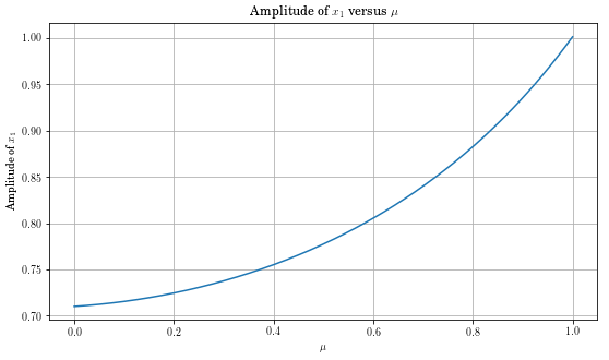
mu = np.linspace(0, 1.0, 200)
amp = np.zeros_like(mu)
for i, mui in enumerate(mu):
    parameters['mu'] = mui
    t, x, e, amps, phases = ms.hb_time(two_dof_coulomb, num_variables=4, omega=1.2,
                                     eqform='first_order', num_harmonics=3, params=parameters)
    amp[i] = amps[0]

Too much Coulomb friction can increase the response.

• Did you know that?

• This damping shifted resonance.

plt.plot(mu,amp)
plt.title('Amplitude of $x_1$ versus $\\mu$')
plt.ylabel('Amplitude of $x_1$')
plt.xlabel('$\\mu$')
plt.grid()

But can I solve an equation in one line? Yes!!!

Damped Duffing oscillator in one command.

out = ms.hb_time(lambda x, v,
               params: np.array([[-x - .1 * x**3 - .1 * v + 1 *
                                  sin(params['omega'] * params['cur_time'])]]),
               num_variables=1, omega=.7, num_harmonics=1)
out[3][0]

1.4779630014433971

OK - that’s a bit obtuse. I wouldn’t do that normally, but Mousai can.

How to get this?

• Install Scientific Python from SciPy.org

  • AFRL: See your tech support to get the Enthought distribution installed

• See the Mousai documents for installation instructions

  • pip install mousai

  • AFRL: Talk to me- install is easy if I send you the files.

• See Mousai on GitHub (https://github.com/josephcslater/mousai)

Conclusions

• Nonlinear frequency solutions are within reach of undergraduates

• Installation is trivial

• Already in use (GitHub logs indicate dozens of users)

• Custom special case and proprietary solvers such as BDamper can be replaced for free

• Research potential is about to be unleashed

Future

• Add time-averaging method

  • currently requires high number of harmonics for non-smooth systems

• Add masking of known harmonics (average is often fixed and known)

• Automated sweep control

• Branch following

• Condense the one-line method

• Evaluate on large scale problems

  • Currently attempting to hook to ANSYS

• Parallelize

• Leverage CUDA