Harmonic Balance Tools (mousai.har_bal)
Harmonic balance solvers and other related tools.
-
har_bal.condense_fft(X_full, num_harmonics)[source]¶ Create equivalent amplitude reduced-size FFT from longer FFT.
-
har_bal.function_to_mousai(sdfunc)[source]¶ Convert scipy.integrate functions to Mousai form.
The form of the function returning state derivatives is sdfunc(x, t, params) where x are the current states as an n by 1 array, t is a scalar, and params is a dictionary of parameters, one of which must be omega. This is inconsistent with the SciPy numerical integrators for good cause, but can make simultaneous usage diffucult.
This function returns a function compatible with Mousai by using the inspect package to determine the form of the function being used and to wrap it in Mousai form.
- Parameters
- Returns
- new_functionfunction
function in Mousai form (accepting inputs like a standard Mousai function)
Notes
See also
old_mousai_to_new_mousaimousai_to_odeintmousai_to_solve_ivp
-
har_bal.harmonic_deriv(omega, r)[source]¶ Return derivative of a harmonic function using frequency methods.
- Parameters
- omega: float
Fundamendal frequency, in rad/sec, of repeating signal
- r: array_like
- Array of rows of time histories to take the derivative of.The 1 axis (each row) corresponds to a time history.The length of the time histories must be an odd integer.
- Returns
- s: array_like
Function derivatives. The 1 axis (each row) corresponds to a time history.
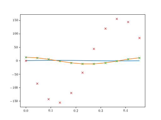
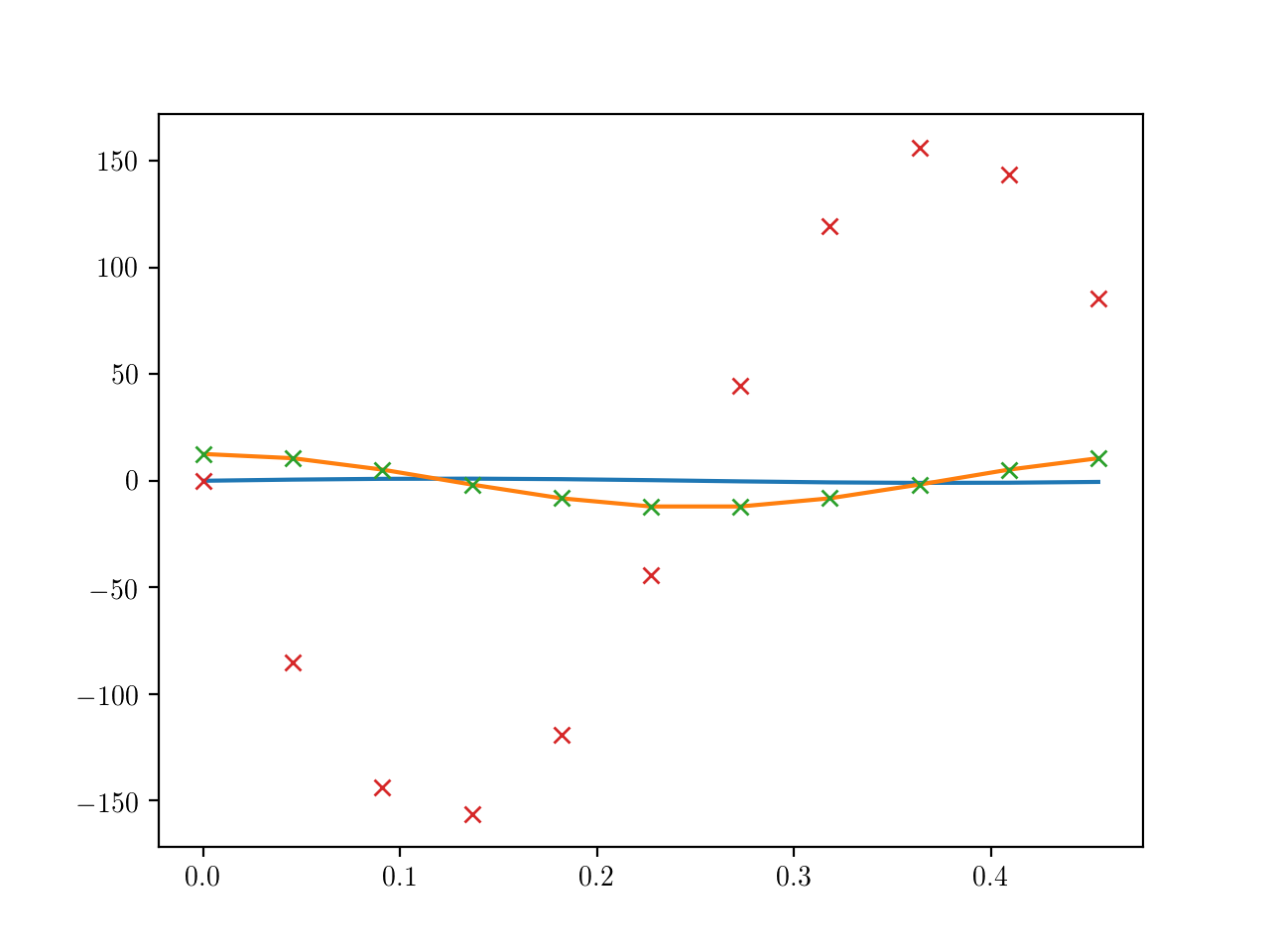
Examples
(Source code, png, hires.png, pdf)
-
har_bal.hb_freq(sdfunc, x0=None, omega=1, method='newton_krylov', num_harmonics=1, num_variables=None, mask_constant=True, eqform='second_order', params={}, realify=True, num_time_steps=51, **kwargs)[source]¶ Harmonic balance solver for first and second order ODEs.
Obtains the solution of a first-order and second-order differential equation under the presumption that the solution is harmonic using an algebraic time method.
Returns t (time), x (displacement), v (velocity), and a (acceleration) response of a first or second order linear ordinary differential equation defined by \(\ddot{\mathbf{x}}=f(\mathbf{x},\mathbf{v},\omega)\) or \(\dot{\mathbf{x}}=f(\mathbf{x},\omega)\).
For the state space form, the function sdfunc should have the form:
def duff_osc_ss(x, params):  # params is a dictionary of parameters
    omega = params['omega']  # `omega` will be put into the dictionary
                             # for you
    t = params['cur_time']   # The time value is available as
                             # `cur_time` in the dictionary
    x_dot = np.array([[x[1]],
                      [-x[0]-.1*x[0]**3-.1*x[1]+1*sin(omega*t)]])
    return x_dot
In a state space form solution, the function must take the states and the params dictionary. This dictionary should be used to obtain the prescribed response frequency and the current time. These plus any other parameters are used to calculate the state derivatives which are returned by the function.
For the second order form the function sdfunc should have the form:
def duff_osc(x, v, params):  # params is a dictionary of parameters
    omega = params['omega']  # `omega` will be put into the dictionary
                             # for you
    t = params['cur_time']   # The time value is available as
                             # `cur_time` in the dictionary
    return np.array([[-x-.1*x**3-.2*v+sin(omega*t)]])
In a second-order form solution the function must take the states and the params dictionary. This dictionary should be used to obtain the prescribed response frequency and the current time. These plus any other parameters are used to calculate the state derivatives which are returned by the function.
- Parameters
- sdfuncfunction
For eqform=’first_order’, name of function that returns column vector first derivative given x, and a dictionry of parameters. This is NOT a string (not the name of the function).
\(\dot{\mathbf{x}}=f(\mathbf{x},\omega)\)
For eqform=’second_order’, name of function that returns column vector second derivative given x, v, omega and **kwargs. This is NOT a string.
\(\ddot{\mathbf{x}}=f(\mathbf{x},\mathbf{v},\omega)\)
- x0array_like, somewhat optional
n x m array where n is the number of equations and m is the number of values representing the repeating solution. It is required that \(m = 1 + 2 num_{harmonics}\). (we will generalize allowable default values later.)
- omegafloat
assumed fundamental response frequency in radians per second.
- methodstr, optional
Name of optimization method to be used.
- num_harmonicsint, optional
Number of harmonics to presume. The omega = 0 constant term is always presumed to exist. Minimum (and default) is 1. If num_harmonics*2+1 exceeds the number of columns of x0 then x0 will be expanded, using Fourier analaysis, to include additional harmonics with the starting presumption of zero values.
- num_variablesint, somewhat optional
Number of states for a state space model, or number of generalized dispacements for a second order form. If x0 is defined, num_variables is inferred. An error will result if both x0 and num_variables are left out of the function call. num_variables must be defined if x0 is not.
- eqformstr, optional
second_order or first_order. (second order is default)
- paramsdict, optional
Dictionary of parameters needed by sdfunc.
- realifyboolean, optional
Force the returned results to be real.
- mask_constantboolean, optional
Force the constant term of the series representation to be zero.
- num_time_stepsint, default = 51
number of time steps to use in time histories for derivative calculations.
- otherany
Other keyword arguments available to nonlinear solvers in scipy.optimize.nonlin. See Notes.
- Returns
- t, x, e, amps, phasesarray_like
time, displacement history (time steps along columns), errors,
- ampsfloat array
amplitudes of displacement (primary harmonic) in column vector format.
- phasesfloat array
amplitudes of displacement (primary harmonic) in column vector format.
Notes
See also
hb_time
Calls a linear algebra function from scipy.optimize.nonlin with newton_krylov as the default.
Evaluates the differential equation/s at evenly spaced points in time defined by the user (default 51). Uses error in FFT of derivative (acceeration or state equations) calculated based on:
governing equations
derivative of x (second derivative for state method)
Solver should gently “walk” solution up to get to nonlinearities for hard nonlinearities.
- Algorithm:
calls hb_time_err with x as the variable to solve for.
hb_time_err uses a Fourier representation of x to obtain velocities (after an inverse FFT) then calls sdfunc to determine accelerations.
Accelerations are also obtained using a Fourier representation of x
Error in the accelerations (or state derivatives) are the functional error used by the nonlinear algebraic solver (default newton_krylov) to be minimized by the solver.
Options to the nonlinear solvers can be passed in by **kwargs.
Examples
>>> import mousai as ms
>>> t, x, e, amps, phases = ms.hb_freq(ms.duff_osc,
...                                    np.array([[0,1,-1]]),
...                                    omega = 0.7)
-
har_bal.hb_time(sdfunc, x0=None, omega=1, method='newton_krylov', num_harmonics=1, num_variables=None, eqform='second_order', params={}, realify=True, **kwargs)[source]¶ Harmonic balance solver for first and second order ODEs.
Obtains the solution of a first-order and second-order differential equation under the presumption that the solution is harmonic using an algebraic time method.
Returns t (time), x (displacement), v (velocity), and a (acceleration) response of a first- or second- order linear ordinary differential equation defined by \(\ddot{\mathbf{x}}=f(\mathbf{x},\mathbf{v},\omega)\) or \(\dot{\mathbf{x}}=f(\mathbf{x},\omega)\).
For the state space form, the function sdfunc should have the form:
def duff_osc_ss(x, params):  # params is a dictionary of parameters
    omega = params['omega']  # `omega` will be put into the dictionary
                             # for you
    t = params['cur_time']   # The time value is available as
                             # `cur_time` in the dictionary
    xdot = np.array([[x[1]],[-x[0]-.1*x[0]**3-.1*x[1]+1*sin(omega*t)]])
    return xdot
In a state space form solution, the function must accept the states and the params dictionary. This dictionary should be used to obtain the prescribed response frequency and the current time. These plus any other parameters are used to calculate the state derivatives which are returned by the function.
For the second order form the function sdfunc should have the form:
def duff_osc(x, v, params):  # params is a dictionary of parameters
    omega = params['omega']  # `omega` will be put into the dictionary
                             # for you
    t = params['cur_time']   # The time value is available as
                             # `cur_time` in the dictionary
    return np.array([[-x-.1*x**3-.2*v+sin(omega*t)]])
In a second-order form solution the function must take the states and the params dictionary. This dictionary should be used to obtain the prescribed response frequency and the current time. These plus any other parameters are used to calculate the state derivatives which are returned by the function.
- Parameters
- sdfuncfunction
For eqform=’first_order’, name of function that returns column vector first derivative given x, and a dictionry of parameters. This is NOT a string (not the name of the function).
\(\dot{\mathbf{x}}=f(\mathbf{x},\omega)\)
For eqform=’second_order’, name of function that returns column vector second derivative given x, v, and a dictionary of parameters. This is NOT a string.
\(\ddot{\mathbf{x}}=f(\mathbf{x},\mathbf{v},\omega)\)
- x0array_like, somewhat optional
n x m array where n is the number of equations and m is the number of values representing the repeating solution. It is required that \(m = 1 + 2 num_{harmonics}\). (we will generalize allowable default values later.)
- omegafloat
assumed fundamental response frequency in radians per second.
- methodstr, optional
Name of optimization method to be used.
- num_harmonicsint, optional
Number of harmonics to presume. The omega = 0 constant term is always presumed to exist. Minimum (and default) is 1. If num_harmonics*2+1 exceeds the number of columns of x0 then x0 will be expanded, using Fourier analaysis, to include additional harmonics with the starting presumption of zero values.
- num_variablesint, somewhat optional
Number of states for a state space model, or number of generalized dispacements for a second order form. If x0 is defined, num_variables is inferred. An error will result if both x0 and num_variables are left out of the function call. num_variables must be defined if x0 is not.
- eqformstr, optional
second_order or first_order. (second order is default)
- paramsdict, optional
Dictionary of parameters needed by sdfunc.
- realifyboolean, optional
Force the returned results to be real.
- otherany
Other keyword arguments available to nonlinear solvers in scipy.optimize.nonlin. See Notes.
- Returns
- t, x, e, amps, phasesarray_like
time, displacement history (time steps along columns), errors,
- ampsfloat array
amplitudes of displacement (primary harmonic) in column vector format.
- phasesfloat array
amplitudes of displacement (primary harmonic) in column vector format.
Notes
See also
hb_freqThis method is not reliable for a low number of harmonics.
Calls a linear algebra function from scipy.optimize.nonlin with newton_krylov as the default.
Evaluates the differential equation/s at evenly spaced points in time. Each point in time yields a single equation. One harmonic plus the constant term results in 3 points in time over the cycle.
Solver should gently “walk” solution up to get to nonlinearities for hard nonlinearities.
- Algorithm:
calls hb_err with x as the variable to solve for.
hb_err uses a Fourier representation of x to obtain velocities (after an inverse FFT) then calls sdfunc to determine accelerations.
Accelerations are also obtained using a Fourier representation of x
Error in the accelerations (or state derivatives) are the functional error used by the nonlinear algebraic solver (default newton_krylov) to be minimized by the solver.
Options to the nonlinear solvers can be passed in by **kwargs (keyword arguments) identical to those available to the nonlinear solver.
Examples
>>> import mousai as ms
>>> t, x, e, amps, phases = ms.hb_time(ms.duff_osc,
...                                    np.array([[0,1,-1]]),
...                                    omega = 0.7)
-
har_bal.mousai_to_odeint(sdfunc, params)[source]¶ Return function callable from solve_ivp given Mousai a sdfunc.
- Parameters
- sdfuncfunction
Mousai-style function returning state derivatives.
- paramsdictionary
dictionary of parameters used by sdfunc.
- Returns
- odeint_functionfunction
function ordered to work with odeint
Notes
See also
function_to_mousaiold_mousai_to_new_mousaimousai_to_solve_ivp
-
har_bal.mousai_to_solve_ivp(sdfunc, params)[source]¶ Return function callable from solve_ivp given Mousai sdfunc.
- Parameters
- sdfuncfunction
Mousai-style function returning state derivatives.
- paramsdictionary
dictionary of parameters used by sdfunc.
- Returns
- solve_ivp_functionfunction
function ordered to work with solve_ivp
Notes
The ability to pass parameters was deprecated in the new SciPy integrators: https://stackoverflow.com/questions/48245765/pass-args-for-solve-ivp-new-scipy-ode-api https://github.com/scipy/scipy/issues/8352
See also
function_to_mousaiold_mousai_to_new_mousaimousai_to_odeint
-
har_bal.old_mousai_to_new_mousai(function)[source]¶ Return derivative function converted to new Mousai format.
The original format for the Mousai derivative function was sdfunc(x, params). This is inconsistent with the SciPy integration functions. To act more as expected, the standard from 0.4.0 on will take the form sdfunc(x, t, params).
- Parameters
- sdfuncfunction
function in old Mousai form. sdfunc(y, params)
- Returns
- new_sdfuncfunction
function in new Mousai form. sdfunc(y, t, params)
Notes
See also
function_to_mousaimousai_to_odeintmousai_to_solve_ivp
-
har_bal.solmf(x, v, M, C, K, F)[source]¶ Return acceleration of second order linear matrix system.
- Parameters
- x, v, Farray_like
\(n\times 1\) arrays of current displacement, velocity, and Force.
- M, C, Karray_like
Mass, damping, and stiffness matrices.
- Returns
- aarray_like
\(n\\times 1\) acceleration vector
Examples
>>> import numpy as np
>>> M = np.array([[2,0],[0,1]])
>>> K = np.array([[2,-1],[-1,3]])
>>> C = 0.01 * M + 0.01 * K
>>> x = np.array([[1],[0]])
>>> v = np.array([[0],[10]])
>>> F = v * 0.1
>>> a = solmf(x, v, M, C, K, F)
>>> print(a)
    [[-0.95]
     [ 1.6 ]]
-
har_bal.time_history(t, x, num_time_points=200, realify=True)[source]¶ Generate refined time history from harmonic balance solution.
Harmonic balance solutions presume a limited number of harmonics in the solution. The result is that the time history is usually a very limited number of values. Plotting these results implies that the solution isn’t actually a continuous one. This function fills in the gaps using the harmonics obtained in the solution.
- Parameters
- t: array_like
1 x m array where m is the number of values representing the repeating solution.
- x: array_like
n x m array where m is the number of equations and m is the number of values representing the repeating solution.
- realify: boolean
Force the returned results to be real.
- num_time_points: int
number of points desired in the “smooth” time history.
- Returns
- t: array_like
1 x num_time_points array.
- x: array_like
n x num_time_points array.
Notes
The implication of this function is that the higher harmonics that were not determined in the solution are zero. This is indeed the assumption made when setting up the harmonic balance solution. Whether this is a valid assumption is something that the user must judge when obtaining the solution.
Examples
>>> import numpy as np
>>> import mousai as ms
>>> x = np.array([[-0.34996499,  1.36053998, -1.11828552]])
>>> t = np.array([0.        , 2.991993  , 5.98398601])
>>> t_full, x_full = ms.time_history(t, x, num_time_points=300)
-
har_bal.time_history_r(t, x, num_time_points=200, realify=True)[source]¶ Generate refined time history from harmonic balance solution.
Harmonic balance solutions presume a limited number of harmonics in the solution. The result is that the time history is usually a very limited number of values. Plotting these results implies that the solution isn’t actually a continuous one. This function fills in the gaps using the harmonics obtained in the solution.
- Parameters
- t: array_like
1 x m array where m is the number of values representing the repeating solution.
- x: array_like
n x m array where m is the number of equations and m is the number of values representing the repeating solution.
- realify: boolean
Force the returned results to be real.
- num_time_points: int
number of points desired in the “smooth” time history.
- Returns
- t: array_like
1 x num_time_points array.
- x: array_like
n x num_time_points array.
Notes
The implication of this function is that the higher harmonics that were not determined in the solution are zero. This is indeed the assumption made when setting up the harmonic balance solution. Whether this is a valid assumption is something that the user must judge when obtaining the solution.
Examples
>>> import numpy as np
>>> import mousai as ms
>>> x = np.array([[-0.34996499,  1.36053998, -1.11828552]])
>>> t = np.array([0.        , 2.991993  , 5.98398601])
>>> t_full, x_full = ms.time_history(t, x, num_time_points=300)