Lab 3: Computation of Rotating Unbalance¶

In [18]:

clear all
close all
clc
imatlab_export_fig('print-png')

In [5]:

% Obtained from curve fitting sdofcf
zeta = 0.0020271;
f = 206.94; % second natural frequency in Hz

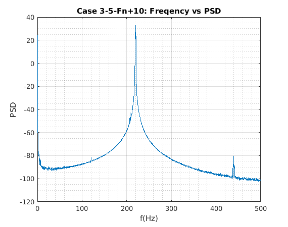
Power Spectrum Density plot¶

In [6]:

load('Case3-5-Fn+10')
figure
A=20*log10(PSD_chan_2);
plot(Freq_domain,A);
grid on
grid minor
title('Case 3-5-Fn+10: Freqency vs PSD')
xlabel('f(Hz)')
ylabel('PSD')

../_images/labnotes_Matlab3_4_0.png

Experimental Data Analysis¶

In [7]:

load('Case3-5-Fn+10')
% Driving Freqency
[x,y]=max(PSD_chan_2);
wr=Freq_domain(y) %in Hz
[a,b]=max(A);


wr =

  single

  219.6875

In [8]:

load('Case3-1')

HI=abs(Hf_chan_2);
h=HI(b)%inertance in 1/kg


h =

  343.3732

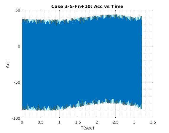
Acceleration Response Plot¶

In [9]:

load('Case3-5-Fn+10')
figure
plot(Time_domain,(Time_chan_2*9.81))
grid on
grid minor
title('Case 3-5-Fn+10: Acc vs Time')
xlabel('T(sec)')
ylabel('Acc')

../_images/labnotes_Matlab3_9_0.png

Data Analysis¶

In [10]:

Amax=max((Time_chan_2*9.81)-1);
Xmax=(Amax)/(wr*2*pi)^2 %max displ


Xmax =

  single

  2.2536e-05

In [11]:

r=wr/f % freq ratio


r =

  single

    1.0616

In [12]:

moe=Xmax/h %experimental rotating unbalance


moe =

  single

  6.5630e-08

Beam Properties¶

In [13]:

l=21.75*0.0254;% length in meters
h=0.5*0.0254;% height in meters
w=1*0.0254;% width in meters
rho=2700;% density in kg/cubicmeter
V = l*w*h;% volume (m^3)
m=rho*V


m =

    0.4812

Analytical rotating unbalance¶

In [14]:

moeA=m*Xmax*sqrt((1-r^2)^2+(2*zeta*r)^2)/(r^2)


moeA =

  single

  1.2226e-06