Lab 1: Identification of Damping Using Log Decrement
In [1]:
%load_ext autoreload
%autoreload 2
import vibration_toolbox as vtb
from vibration_toolbox import time_plot
import matplotlib.pyplot as plt
import numpy as np
import scipy.io as sio
import math as math
Interactive iPython tools will not work without IPython.display           and ipywidgets installed.
Interactive iPython tools will not work without IPython.display           and ipywidgets installed.
Beam Properties
In [2]:
l=21.75*0.0254;# length in meters
h=0.5*0.0254;# height in meters
w=1*0.0254;# width in meters
rho=2700;# density in kg/cubicmeter
E=7.31e10;# youngs modulus in Pa
I = (1/12)*w*h**3; # moment of inertia (m^4)
k = (3*E*I)/l**3; # stiffness (N/m)
V = l*w*h;# volume (m^3)
m = rho*V;# mass (kg)
wn = math.sqrt(k/m) # analytical natural frequency of massless beam with concentrated mass
wn2=(1.875)**(2)*math.sqrt((E*I)/(m*(l)**3)) #natural freqency of a uniform section beam
#c_cr = 2*math.sqrt(k*m); # critical damping coefficient
In [3]:
wn
Out[3]:
108.259140771331
In [4]:
wn2
Out[4]:
219.7386705465195
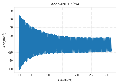
Acceleration vs Time plot
In [5]:
# Acc vs Time

%matplotlib inline
mat_contents=sio.loadmat('Case1-2.mat')
Time_domain = mat_contents['Time_domain']
Time_chan_2 = mat_contents['Time_chan_2']
Time_chan_2 = Time_chan_2*(9.81);
mean=sum(Time_chan_2)/np.size(Time_chan_2);
Accel = Time_chan_2-mean;
# The acceleration values from Bobcat will be in Gs. So,  to convert them to m/s^2,
# we will have to multiply the vector by 9.81
plt.plot(Time_domain, Accel)
plt.grid('on')
plt.ylabel('$Acc(m/s^2)$')
plt.xlabel('$Time(sec)$')
plt.title('$Acc$ versus $Time$')
Out[5]:
<matplotlib.text.Text at 0x7f719edf9438>
Data Analysis ——————–
In [6]:
# Enter values from plots for calculations. Use data cursor to
# obtain x and t values.
x1 = 81.45;
t1 = 0.007031;
x2 = 15.44;
t2 = 3.181;
n = 106;
time = t2-t1;
Log Decrement Method
In [7]:
d = (1/n)*math.log(x1/x2) # delta
d
Out[7]:
0.015688941419353057
In [8]:
z= d/np.sqrt(4*math.pi**2+d**2) # zeta
z
Out[8]:
0.0024969647946533331
In [9]:
Td = (time/n)#damped time period
Td
Out[9]:
0.029943103773584907
In [10]:
wd = 2*math.pi/Td #damped natural frequency
wd
Out[10]:
209.83747559003763
In [11]:
wne = wd/np.sqrt(1-z**2) # natural frequency in rad/sec
wne
Out[11]:
209.83812974392472
In [12]:
k2=(wne**2)*m # one way to use experimental zeta and nat freq to calculate C
k2
Out[12]:
21186.684200875719
In [13]:
c_cr = 2*np.sqrt(k2*m) # critical
In [14]:
c=c_cr*z # damping constant
c
Out[14]:
0.50422108345689065
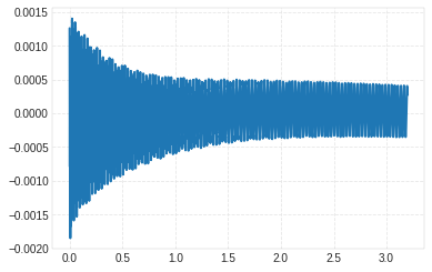
In [15]:
x = Accel*(1/-(wd**2))
x[0]
Out[15]:
array([ 0.00126369], dtype=float32)
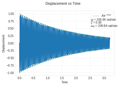
Using Vibration toolbox for comparison
In [30]:
%matplotlib inline
mat_contents=sio.loadmat('Case1-2.mat')
Time_domain = mat_contents['Time_domain']
Time_chan_2 = mat_contents['Time_chan_2']
Time_chan_2 = Time_chan_2*(9.81);
mean=sum(Time_chan_2)/np.size(Time_chan_2);
Accel = Time_chan_2-mean;
ax=max(x);
x = Accel*(1/-(wd**2))# max amplitude
initialvel=-ax*wne;
plt.figure()
vtb.time_plot(m=rho*V, c=c_cr*z, k=(wne**2)*m, x0=0.00126369, v0=-ax*wne, max_time=3.2)
#ax=fig.add_subplot(111)
plt.plot(Time_domain, x)
#grid minor
#plt.title('Case 2: position vs time')
#plt.xlabel('t(s)')
#plt.ylabel('Position (m)')
#plt.legend('Estimated Displacement','Experimental Displacement')
#x[0]
<matplotlib.figure.Figure at 0x7f719ece0320>
Out[30]:
[<matplotlib.lines.Line2D at 0x7f719ea01438>]
In [25]:
[t,x,v,zeta,omega,omega_d,A]=vtb.free_response(m=rho*V, c=c_cr*z, k=(wne**2)*m, x0=0.00126369, v0=-ax*wne, max_time=3.2);
In [26]:
zeta
Out[26]:
0.0024969647946533327
In [27]:
omega
Out[27]:
209.83812974392472
In [28]:
omega_d
Out[28]:
209.83747559003763
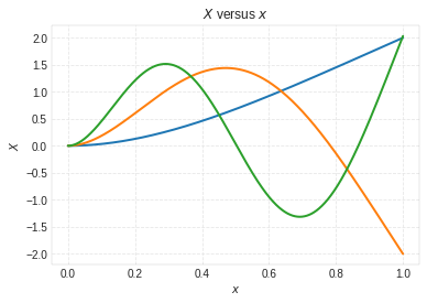
3 Mode shapes
In [29]:
# first three mode shapes
%matplotlib inline
beta = np.array([1.87510407, 4.69409113, 7.85475744])
alpha = np.array([0.7341, 1.0185, 0.9992])
x = np.linspace(0, 1, num=1000)
for i in range(0, 3):
    X=np.cosh(beta[i]*x)-np.cos(beta[i]*x)-alpha[i]*(np.sinh(beta[i]*x)-np.sin(beta[i]*x))
    plt.plot(x, X)
    plt.grid('on')
    plt.ylabel('$X$')
    plt.xlabel('$x$')
    plt.title('$X$ versus $x$')